In this blog post we are going to explain the idea behind making this audio:

sound like this:

The difference you can hear is from a process we have developed called Spectral Recovery.

What is frequency and what is a spectrogram?

To comprehend the importance of frequency recovery, we must first understand what frequency means in the context of audio. While the dictionary definition of frequency describes how often an event occurs within a specific time period, such as someone visiting the gym five times a week, frequency in audio signals is slightly different.

In audio, frequency refers to the repetition rate of a particular sine wave per second. This raises another question: what is a sine wave? A sine wave represents the oscillation pattern of vibrating air molecules, producing a sound similar to a whistle. However, this is just an approximation, as pure sine waves do not exist in real-world audio. The closest sound to a pure sine wave would be that generated by a tuning fork—an intriguing object you might have encountered in a high school physics class. When a tuning fork is struck, it vibrates at a specific frequency—typically 440 Hz for musical applications. If we were to record one second of the sound produced by the vibrating tuning fork, the resulting waveform would look something like this:

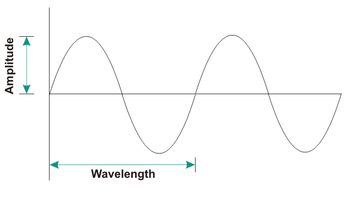
Upon closer examination, we can observe that the wavelength repeats 440 times within the one-second duration.

Listen to the following audio sample:

The audio clip provided was generated by a computer using the equation:

$S = A \cdot \sin (2 \cdot \pi \cdot f \cdot t)$

where $A$, $f$ and $t$ represent amplitude, frequency, and playing time, respectively.

As previously mentioned, pure sine waves do not exist in the physical world. Consequently, a tuning fork’s waveform would look more like this:

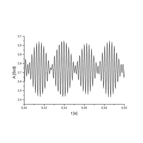
Upon observation, we can see that the image displays a waveform composed of more than a single sine wave. So, how do we determine which frequencies are present in this waveform? The answer lies in using a function called the Fourier Transform.

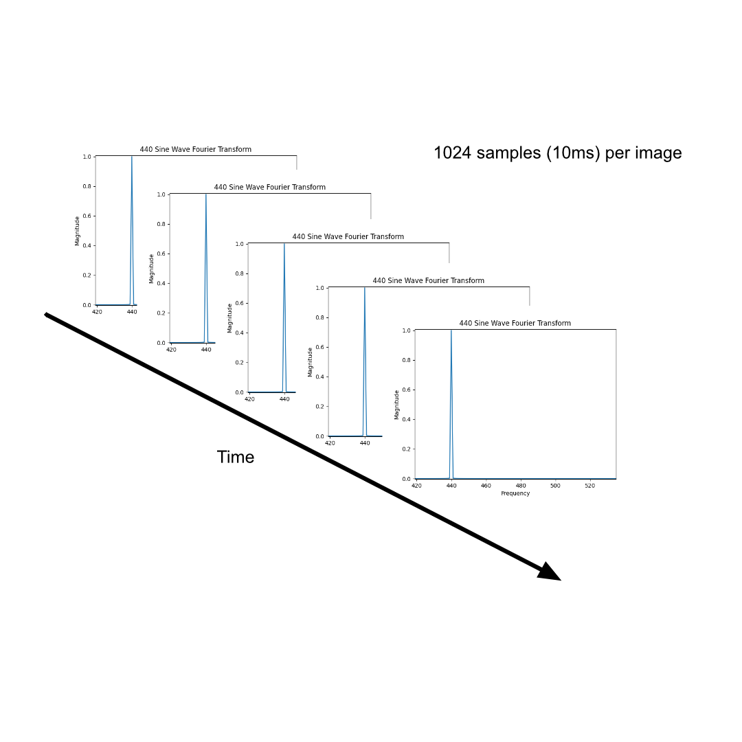
The Fourier Transform (FT) is a powerful tool for breaking down a signal into its individual frequency components. Returning to the 440 Hz sine wave example, if we apply the FT to it, we will find that there is only one component at 440 Hz:

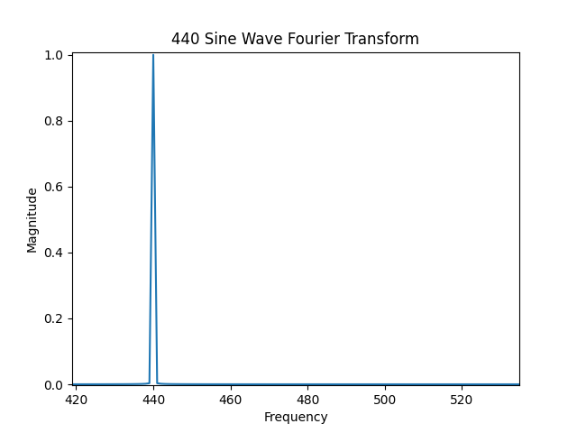
The image was generated by processing a block of $N$ data points, where $N$ is typically a power of 2, such as: 128, 256, 512, 1024, etc.

But what if we need to analyze a continuous sound that could last for hours? The solution is fairly straightforward: we take blocks of a fixed number of samples and repeatedly plot them within a single image. This resulting visualization is called a spectrogram:

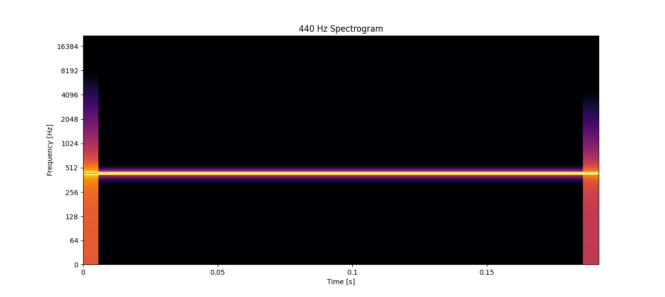
Spectrograms often incorporate color to represent amplitude, adding an extra layer of information to the 2-dimensional graphic. The brighter the color, the higher the amplitude. In the following image, we can see the spectrogram of a 440 Hz frequency captured within approximately 0.20 seconds of audio:

Band-limited signals

To understand why frequency recovery is crucial, we will explain a bit about band-limited signals.

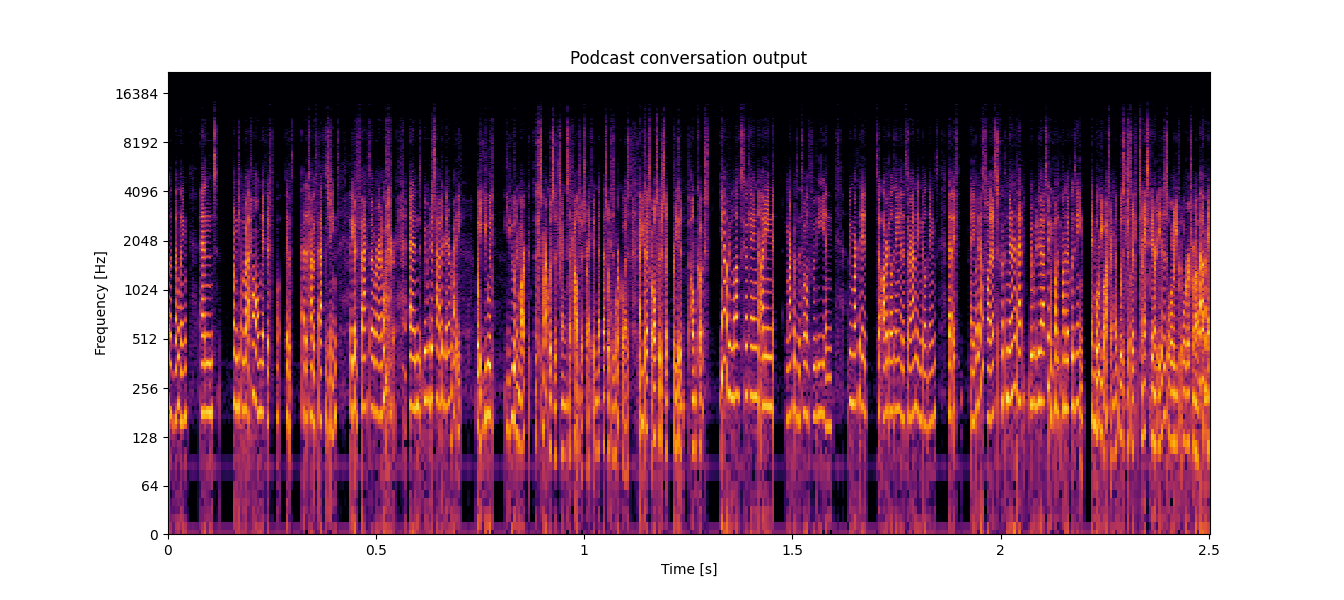
A signal is considered band-limited if, in the spectrogram, there is an abrupt change from a bright color to black, and this black area remains for the duration of the audio file. For instance, phone call audio is typically band-limited to 4 kHz. Take a look at the following figure from a podcast recording with band-limited audio:

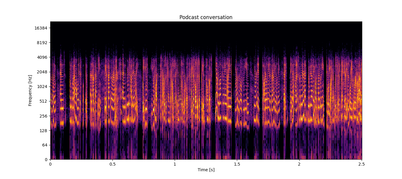
In the spectrogram, we can observe that after 4,000 Hz, there is only black throughout the entire file. This indicates that the signal is band-limited. Band-limited audio lacks many of the characteristics that make it pleasant and rich-sounding to the human ear. Listen to the audio of the spectrogram above:

Humans are capable of perceiving frequencies in the range of 20 Hz to 20,000 Hz. If a sound is band-limited to a frequency below 8,000 Hz, it will be immediately noticeable. For example, when you speak to someone on the phone, the signal is band-limited to 4,000 Hz. Old recordings of songs and speeches are other examples of band-limited audio.

For a sound to be pleasant to the human ear, it should not be band-limited or, at the very least, have a limit of 20,000 Hz.

Frequency recovery

When a band-limited signal is processed to extend its frequency range or increase its resolution beyond its current limit, this is called upsampling.

We previously explained that frequency refers to the number of times a signal occurs in one second. It’s important to distinguish this from the concept of sampling rate, which is the number of points (a.k.a samples) per second used to represent a signal. By understanding both frequency and sampling rate, we can better grasp the nuances of audio processing and analysis.

When we have 8,000 samples in one second, the sampling rate is 8,000 Hz. So, when we discuss frequency recovery, it means converting a low sampling rate (for example, 8,000 Hz) to a higher sampling rate (for example, 44,100 Hz).

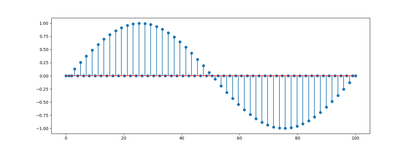
To achieve this, one basic upsampling algorithm involves inserting a series of zeros between each sample of the original signal. Consider the following signal

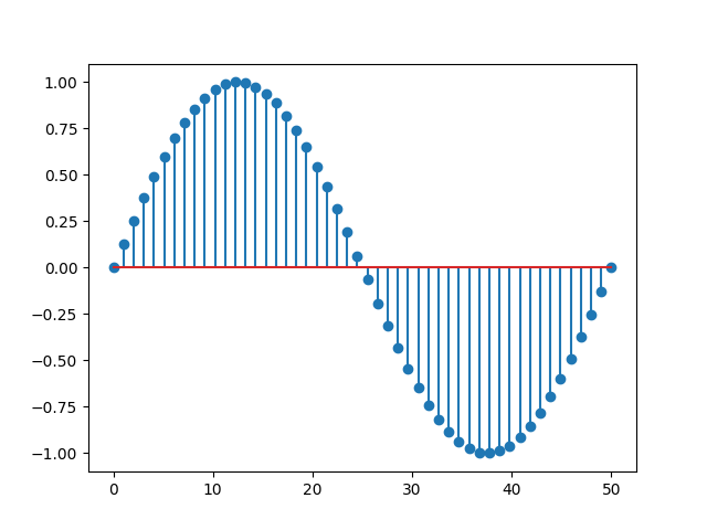
By adding a zero between each sample, the resulting signal will have twice the number of samples as the original one, effectively doubling the sampling rate.

Once the signal has doubled in length, we need to adjust the added zeros to values close to their adjacent values. The simplest way to do this is by applying a low-pass filter to the signal as shown below:

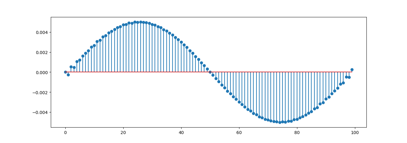
However, this method is prone to errors and does not reliably generate high frequencies necessary for achieving a high-quality sound.

Consider the situation when you have a low-quality image on your phone and you want to zoom in. No matter how much you zoom in, the quality of the image will remain the same, despite the processing your phone does to enlarge the image.

Now, listen to the following examples: one is sampled at 8,000 Hz (similar to phone call quality), and the other is the same audio but upsampled to 44,100 Hz (44.1 kHz is the standard for good quality audio):

Can you tell the difference? The answer would likely be no, because upsampling simply enlarges the waveform, but does not significantly improve the audio’s quality.

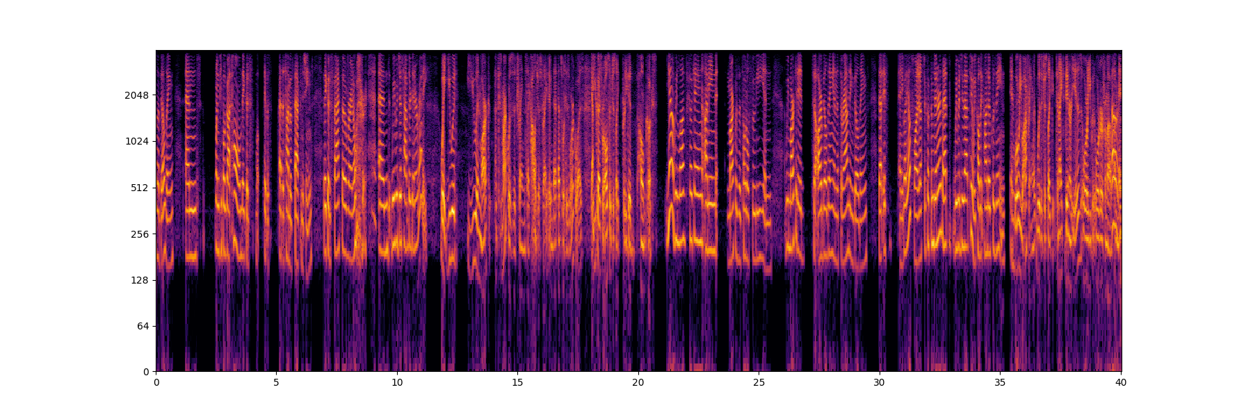
When we examine the spectrogram of audio sampled at a rate of rs = 8,000 Hz, we can see that it includes frequencies up to rs / 2. This specific frequency is called the Nyquist frequency. The Nyquist theorem states that the maximum frequency we can hear is rs / 2. The following figure shows the spectrogram up to only rs / 2, since the other part is symmetric (you can read about FFT symmetry properties):

Now, let’s take a look at the spectrogram of the upsampled signal:

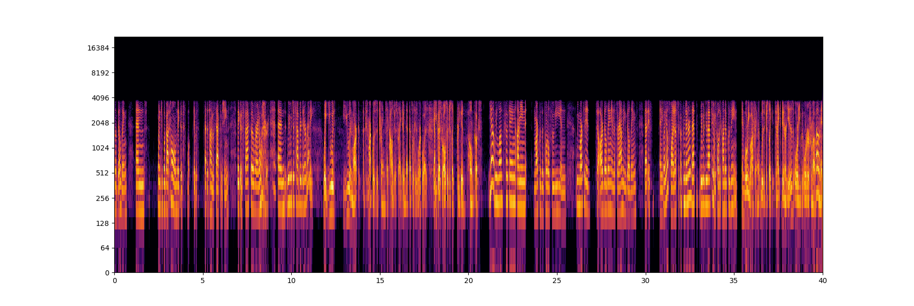
Upon examining the spectrogram of the upsampled signal, we can see that there is no information above 4,000 Hz, even though the new sampling rate is 44,100 Hz. This is because we only enlarged the signal, but we did not process it to include the high frequencies that would make the audio sound better.

By adding zeros, we increased the length; however, to transition from 8,000 Hz to 44,100 Hz, we need to add several zeros between the signal samples and then apply a low-pass filter. There are alternative approaches to assigning values to the zeros between samples, such as linear interpolation or splines, as well as probabilistic methods like Hidden Markov Models.

More complex systems often employ AI to predict the high frequencies. This is where the WAVESHAPER process is applied to upsample and recover the high frequencies of band-limited audio. WAVESHAPER AI models run in real time and deliver high-quality audio.

Listen to the following audio file, which presents the original audio sampled at 8,000 Hz (left) and the audio after our spectral recovery (right); you can hear both the low and high frequencies added to it:

If we examine the spectrogram of the audio file after applying the WAVESHAPER AI’s process, we can see that we have successfully added those missing frequencies: